Slime Simulation

Project Description

My first attempt at GPGPU, simulating the acellular slime mold species, Physarum Polycephalum. The main goal is to demonstrate how complexity in life can arise from following a few simple rules.

This attempt was heavily inspired by Sebastian Lague's coding adventure "Ant & Slime Simulations".

Technologies Used

Process

Given how complex simulating life appeared, it was rather surprising for me to realise the simplistic rules that govern this simulation. The simulated organism essentially follows a simple algorithm: it secretes a trail of pheromones as it moves, tends to move in the same direction it was previously moving, and prefers to follow its nose to areas of higher pheromone concentration.

This particular implementation has 250000 agents and could easily be run on a GPU due to its highly parallel nature. Each agent operates independently, making decisions based on its local environment, which leads to a beautiful emergent behavior when viewed as a whole. The simulation also includes an evaporation and diffusion process for the pheromones, further contributing to the complexity of the system.

Usually I would do this in compute shaders but since I want this to be web friendly, I’ve taken the approach of using ping-pong texture computing where one texture is used as the read buffer and the other one as the output buffer. After each computation cycle, the buffers swap places with each other. In pseudocode code, it looks something like this:

For each agent:
    Read current pheromone value from texture A
    Write the updated pheromone value to texture B
Swap textures A and B
Repeat

Agent Computation

In our case, an agent has 2 properties, a position vector and a normalised direction vector stored in a vec4’s xy and zw components respectively. We can then calculate the angle theta with respect to the positive x-axis which will allow me to apply rotations by simply adding or subtracting from theta.

float theta = atan(direction.y, direction.x);

Now in addition to moving in a straight line, each agent will tend to deviate from its original path

This deviation is determined by a random value, 'wander', which is assigned a value between -1.0 and 1.0. This will then be added to the current direction, causing the agent to wander in a random direction within a given range.

float wander = random() * 2.0 - 1.0;

Now each agent has 3 separate sensors

Each sensor reads the pheromone level at its location, and the agent uses this information to decide its next direction. The sensor detecting the highest pheromone concentration will determine the agent's new direction, drawing it towards areas with more pheromones.

vec2 sensorLeftPosition = position + uSensorOffset*vec2(cos(theta + uSensorAngle), sin(theta + uSensorAngle));
vec2 sensorMiddlePosition = position + uSensorOffset*vec2(cos(theta), sin(theta));
vec2 sensorRightPosition = position + uSensorOffset\*vec2(cos(theta - uSensorAngle), sin(theta - uSensorAngle));

vec4 leftSample = texture(uPheromones, (sensorLeftPosition) / uScreenSize);
vec4 middleSample = texture(uPheromones, (sensorMiddlePosition) / uScreenSize);
vec4 rightSample = texture(uPheromones, (sensorRightPosition) / uScreenSize);

float steer = 0.0;
if (length(leftSample) > length(middleSample) && length(leftSample) > length(rightSample)) {
steer = uSteerAngle;
}
if (length(rightSample) > length(middleSample) && length(rightSample) > length(leftSample)) {
steer = -uSteerAngle;
}

Now we can determine the final theta value with the following process

theta += uWanderStrength * wander;
theta += steer;

By adding the velocity to the position, we can get the position for the next frame

float speed = max(uSpeed, 0.001);
vec2 velocity = vec2(speed * cos(theta), speed *sin(theta));

// add velocity to position
position += velocity;

Pheromone Diffusion and Evaporation

The diffusion step involves a gaussian blur and the evaporation step then reduces the pheromone concentration by a small amount, representing the natural decay of pheromones over time. This process allows older trails to fade away, making room for new pathways to be explored.

void main(){
  vec2 uv = gl_FragCoord.xy / uScreenSize;
  vec4 s1 = texelFetch(uTexture, ivec2(gl_FragCoord.xy + vec2(-1,-1)),0);
  vec4 s2 = texelFetch(uTexture, ivec2(gl_FragCoord.xy + vec2( 0,-1)),0);
  vec4 s3 = texelFetch(uTexture, ivec2(gl_FragCoord.xy + vec2( 1,-1)),0);
  vec4 s4 = texelFetch(uTexture, ivec2(gl_FragCoord.xy + vec2(-1, 0)),0);
  vec4 s5 = texelFetch(uTexture, ivec2(gl_FragCoord.xy), 0);
  vec4 s6 = texelFetch(uTexture, ivec2(gl_FragCoord.xy + vec2( 1, 0)),0);
  vec4 s7 = texelFetch(uTexture, ivec2(gl_FragCoord.xy + vec2(-1, 1)),0);
  vec4 s8 = texelFetch(uTexture, ivec2(gl_FragCoord.xy + vec2( 0, 1)),0);
  vec4 s9 = texelFetch(uTexture, ivec2(gl_FragCoord.xy + vec2( 1, 1)),0);

  vec4 blur = (s1 + 2.0 * s2 + s3 + 2.0 * s4 + 4.0 * s5 + 2.0* s6 + s7 + 2.0 * s8 + s9) / 16.0;

  float strength = length(blur.xyz);
  fColor = vec4(blur.xyz * float(strength > 0.0005),1) * (1.0-uDiffusionStrength*0.1);
}

Results

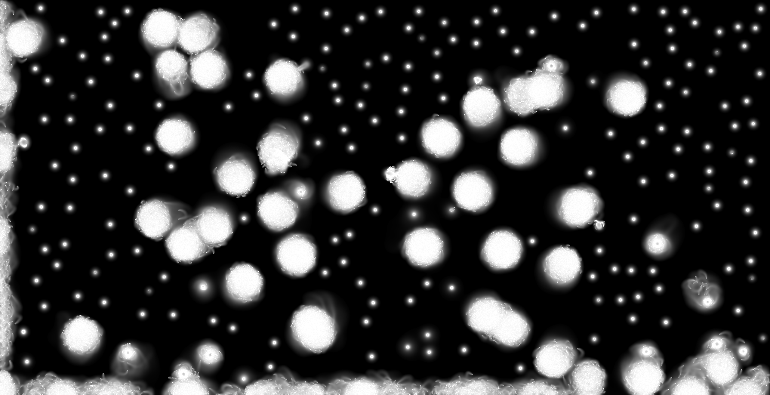
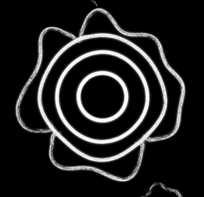
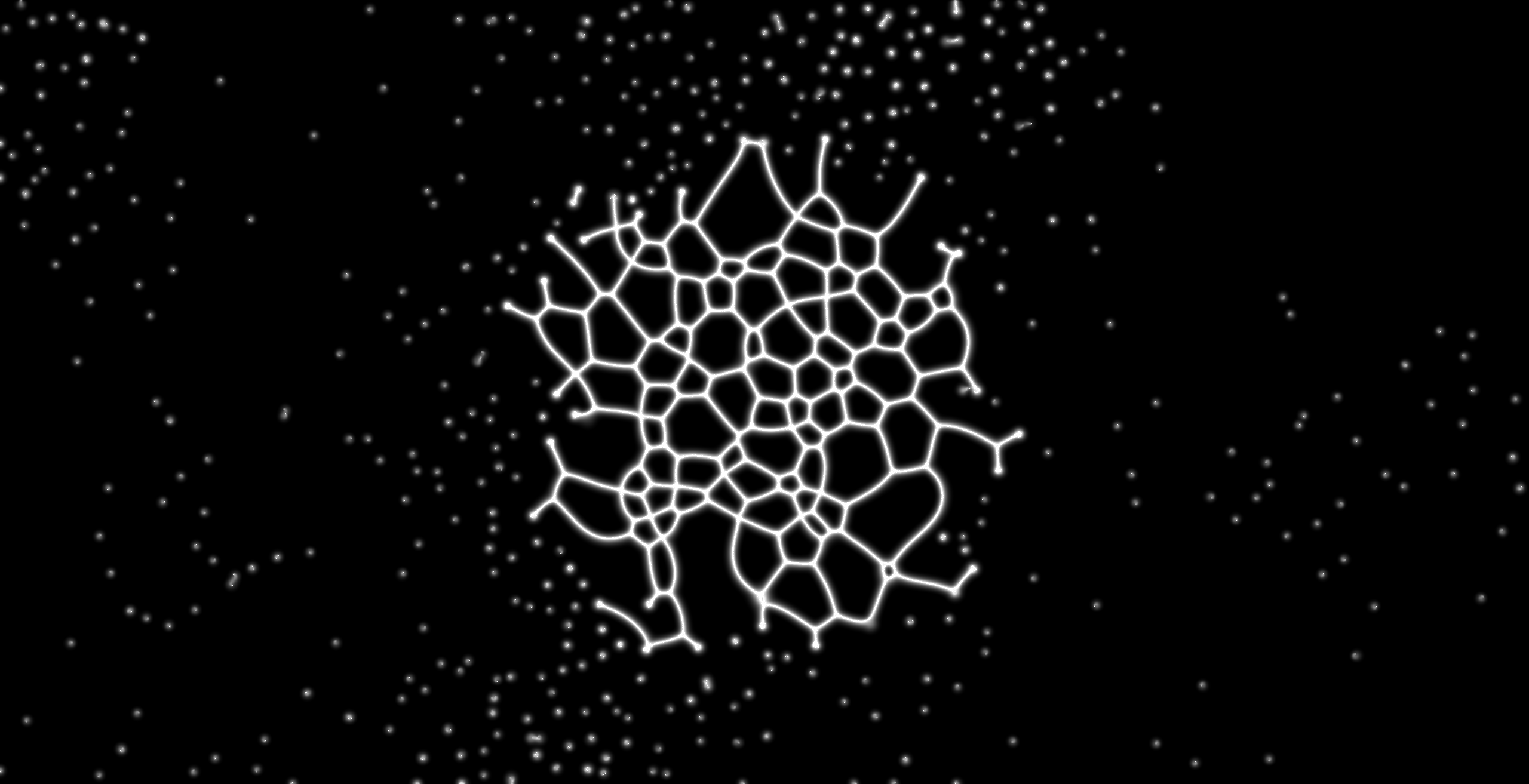
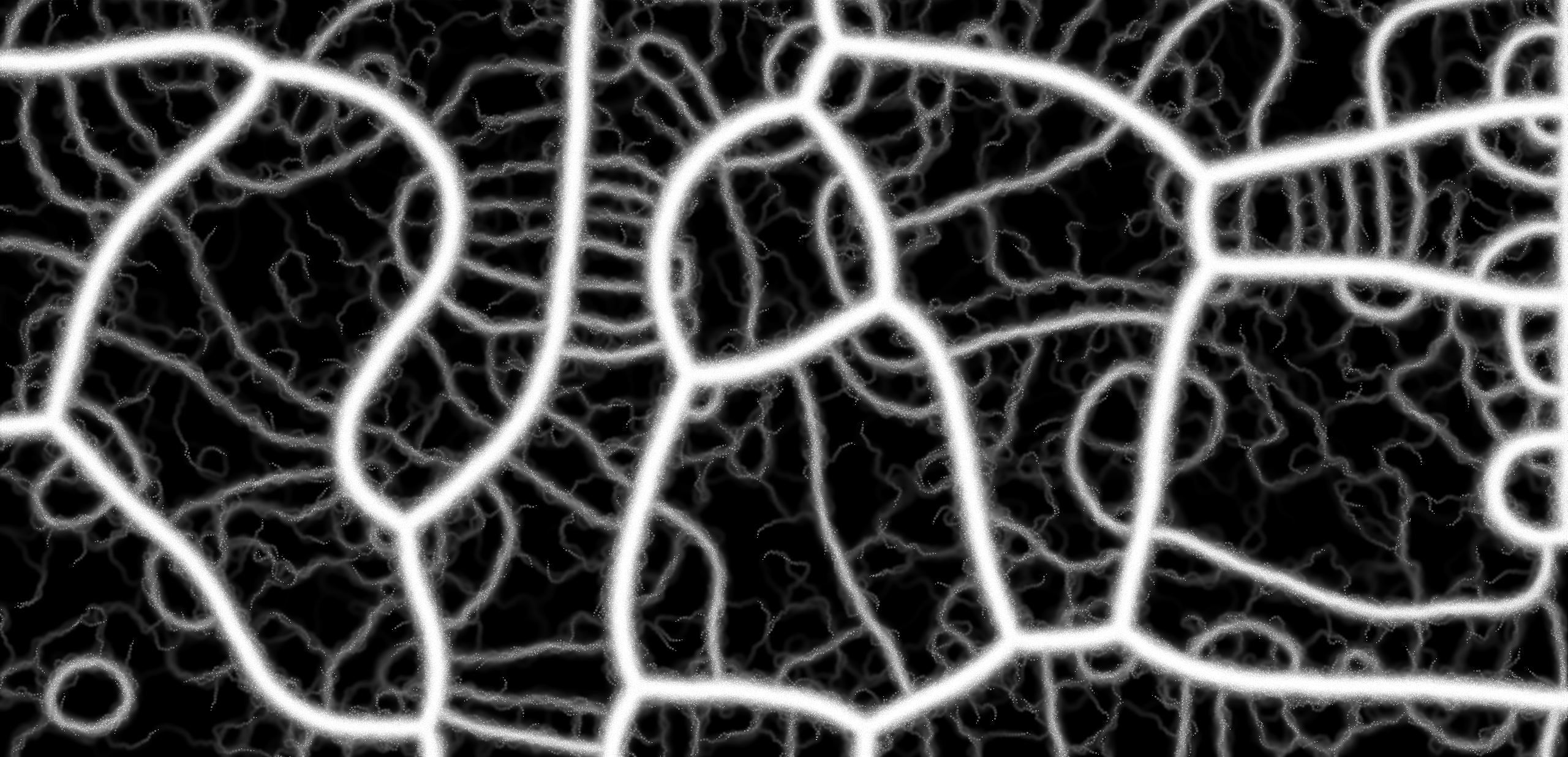
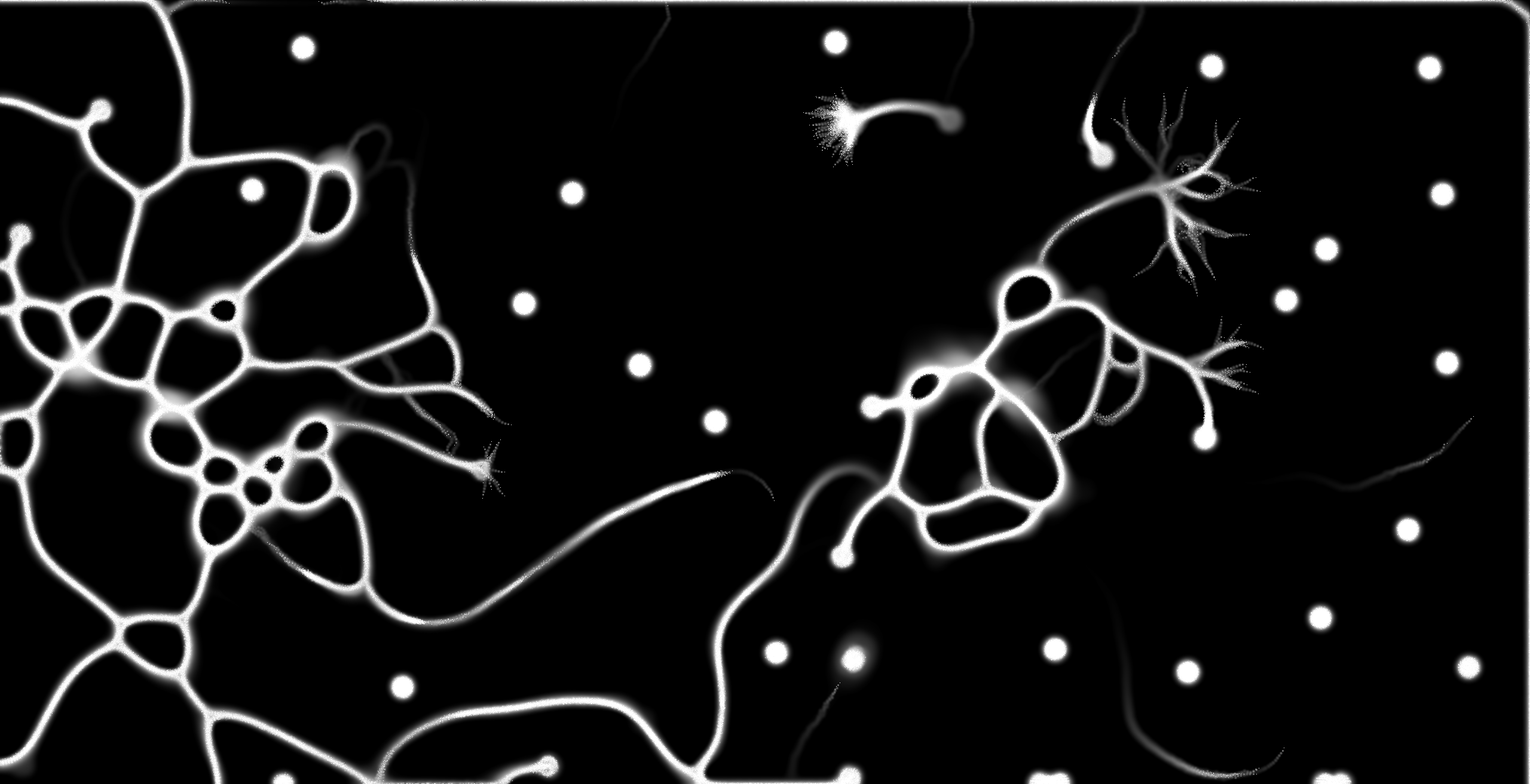
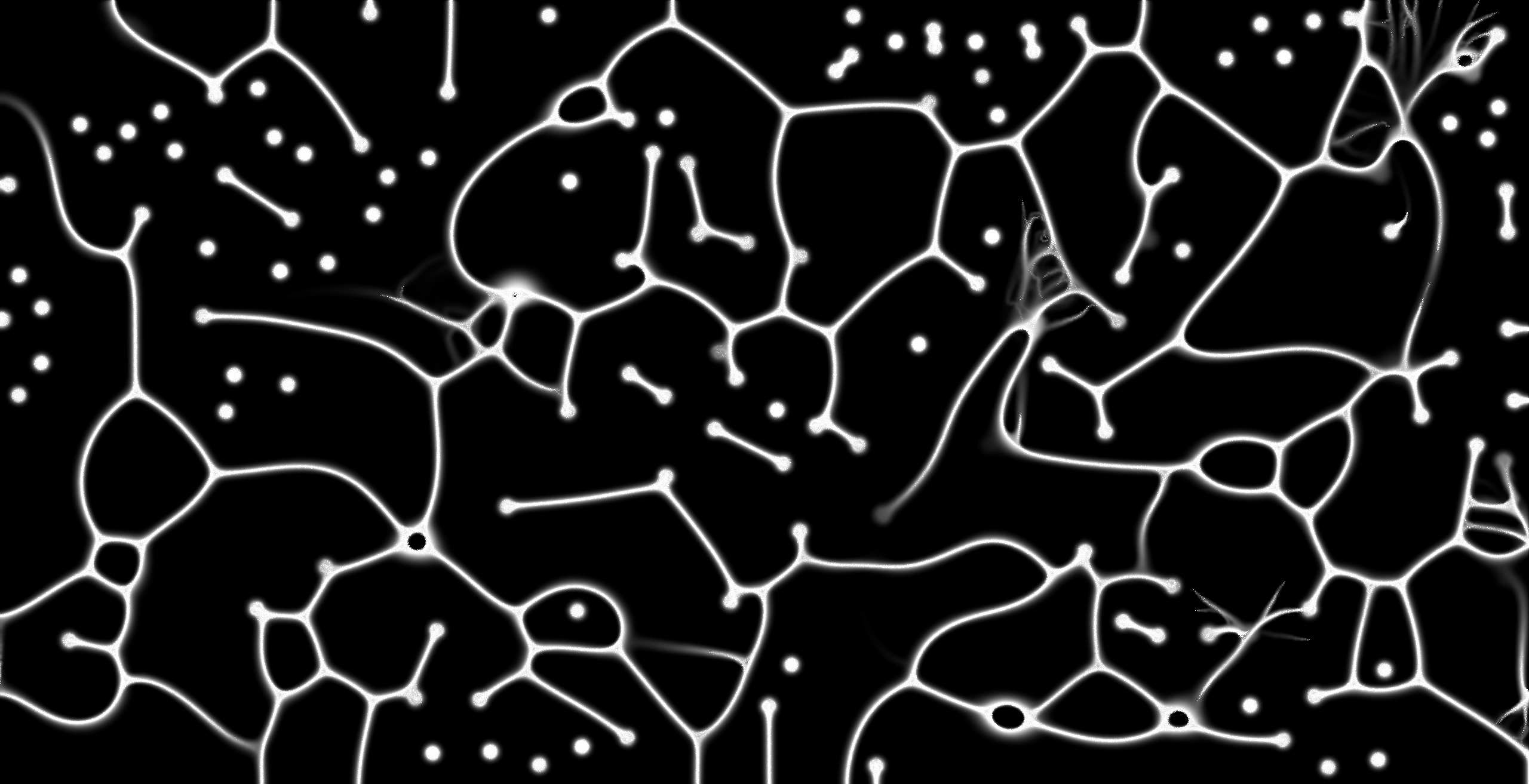
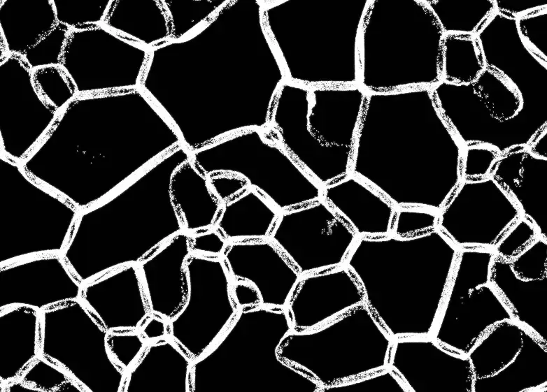
The results were quite beautiful despite the simplistic rules that were given to the program. I have provided a link to the program and I encourage you to check it out as the lossy compression for webp images lowers the detail that I can show you on this blog.